QuEst: Blending Data and Predictions for Robust Quantile Estimation

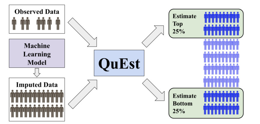
Imagine you track your morning commute times by recording 50 real-world trips with your GPS-enabled phone. You also run a traffic simulator to generate 5,000 possible commute scenarios. You want a reliable estimate of the 95th percentile of commute time—the duration you won’t exceed 95% of the days. Using only your 50 recorded trips yields a wide confidence interval. Using only the simulator risks systematic biases: it might ignore sudden road closures or special events.

QuEst (Quantile-based Estimation) smartly combines both sources:

• It computes the 95th percentile on the real data and on the simulated data.
• It subtracts the simulator’s estimate on just those 50 simulation runs, canceling out any systematic offset.
• It mixes the two estimates with a weight $\lambda$, chosen to minimize the overall sampling variance.

The result is an unbiased, precise estimate of the 95th percentile commute time, with a narrower confidence band than using either source alone.

What Is the QuEst Method?

QuEst estimates any quantile-based measure $Q_{\psi }(F)={\int }_0^1\psi (p)F^{-1}(p)dp$, where $\psi$ is a weight function (e.g., a delta for a single percentile, or a step for CVaR). It leverages:

1. A small set of gold-standard observations ($n$ samples, empirical CDF $F_n$).
2. A large set of model-generated imputations ($N$ samples, empirical CDF ${\hat{F}}_N^e$).

The QuEst estimator is enumerator:

where $F_n^e$ is the simulator’s CDF on the gold sample. This form ensures unbiasedness even if the simulator is biased.

Why Does It Work and Avoid Bias?

1. Bias cancellation: Subtracting the simulator’s estimate on the same sample removes any constant offset.
2. Optimal weight: The weight ${\lambda }^{\ast }$ minimizes asymptotic variance: $${\lambda }^{\ast }=\frac{\mathrm{Cov}(Q_{\psi }(F_n),Q_{\psi }(F_n^e))}{(1+n/N)\mathrm{Var}(Q_{\psi }({\hat{F}}_N^e))}.$$ Empirically, if simulator outputs poorly correlate with real data, ${\lambda }^{\ast }\to 0$, and QuEst defaults to the gold data estimate.

How Does QuEst Self-Correct?

• It estimates variances and covariances from data to choose $\lambda$.
• In an extended version, it parametrizes the weight function $\psi$ as a combination of basis functions and solves a convex optimization to further reduce variance.
• When new real observations arrive, it updates variance estimates, re-computes $\lambda$, and adjusts itself online.

Practical Example: Estimating the 90th Percentile of Website Load Time

Let’s walk through a concrete numeric example using QuEst formulas. Suppose:

• You collect $n=100$ real measurements of page load time, yielding a 90th percentile estimate $Q(F_n)=2.5$ and sample variance 0.04.
• You generate $N=10000$ model-based imputations, giving $Q({\hat{F}}_N^e)=2.3$ and variance 0.01.
• On the same 100-sample subset of imputations, you compute $Q(F_n^e)=2.4$.
• The covariance between the two estimates is 0.02.

1. Compute optimal weight ${\lambda }^{\ast }$:

   $${\lambda }^{\ast }=\frac{0.02}{(1+100/10000)\times 0.01}\approx \mathrm{1.98.}$$

   In practice, cap ${\lambda }^{\ast }$ at 1, so ${\lambda }^{\ast }=1$.

2. Form the QuEst estimator:

   $${\hat{Q}}_{0.9}(\lambda )=\lambda \times 2.3+(2.5-\lambda \times 2.4)=2.3+0.1=\mathrm{2.4.}$$

3. Interpretation:

   • Pure data-only estimate: 2.5 s (high variance).
   • Pure-model estimate: 2.3 s (potential bias).
   • QuEst combined estimate: 2.4 s (bias canceled, variance minimized).

This numeric example shows how to plug observed quantiles, variances, and covariances into QuEst’s formulas to obtain a corrected, low-variance estimate.

📎 Links

• Based on the publication 📄 2507.05220